THIS IS A LEGACY PAGE
We haven't done any work on this in years.
Anyone interested in a low-cost VNA should probably consider a "NanoVNA", which has been out since about 2019.
These can be bought for between $50 and $150 and work amazingly well from about 50 kHz to 1.5 GHz (depending on version).
Low Cost Microwave Network Analyzer
In today’s high technology market, manufacturers are looking to build better products for wireless applications such as mobile phones, pagers and cordless equipment. All of these products require high frequency components for their circuitry. High frequency components benefit from high quality factor characteristics and excellent microwave performance. Testing of these high frequency components requires a Microwave Network Analyzer.
Unfortunately, a modern Microwave Network Analyzer costs around $45,000 or more. For example, the Agilent 8720ES S-parameter Vector Network Analyzer costs $68,245. To generate such large amount of funding is a major obstacle for many microwave circuit researchers and designers at engineering colleges throughout the country. We found there is an alternative way to own a similar set of instruments with about one tenth of the funding. This older set of instruments is built in the pre-computer era, which lacks the computer processor unit. This set of instruments consist of an HP 8350A/B Sweep Oscillator Mainframe with HP 862XXA RF Plug-ins, an HP 8410B Network Analyzer with HP8414A Polar Display Plug-in, an HP 8743B Transmission-Reflection Test Unit with HP 8411A Harmonic Frequency Converter, a National Instrument PCI-6024E data acquisition (DAQ)card, and a personal computer with LabVIEW 6i. With the help of a LabVIEW VI program, calibration correction factors can be applied, accomplishing the same task as the modern network analyzer, but at very low cost.
Block Diagram of a Low Cost Microwave Network Analyzer System [1]
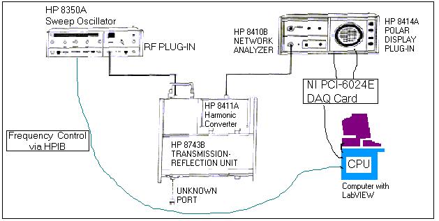
Figure 1
Note: HPIB stands for Hewlett-Packard Interface Bus. The new replacement for HPIB is the GPIB or IEEE488. GPIB stands for General Purpose Interface Bus.
To create an accurate Network Analyzer using low cost available equipment in our laboratory was the main purpose of our project. Before performing measurement of the device under test, a calibration procedure is used to characterize the errors created by the effects of the connectors, cables, and directional couplers within the analyzer. We used our LabVIEW program to perform SHORT, OPEN, and LOAD (SOL) calibrations for the HP 8410B Network Analyzer. After the calibrations, we then make measurements for our device under test. The measured data is corrected according to the calibration data and then displayed on a Smith Chart on the LabVIEW front panel.
|
LabVIEW Front Panel and Block Diagram LabVIEW is a useful instrumentation and analysis software developed by National Instruments. It stands for Laboratory Virtual Instrument Engineering Workbench [2].
VIs are combination of a Front Panel and Block Diagram (see Figure 2 above). LabVIEW VIs can used within other Vis as sub-Vis because they are hierarchical and modular. In other words, one can use them as top-level programs, or as subprograms within other programs (see Figure 3). Sub-VI |
As we perform the SOL calibration, we control the frequencies of the HP 8350 Sweep Oscillator by the LabVIEW program via the HPIB interface (see figure 1). In the LabVIEW program, the user selects how many data points and what frequency range he or she wants to display the output on the Smith Chart. The data is collected as the frequencies advance through the user-specified range in the Sweep Oscillator.
As the SOL data are collected, we store them in three LabVIEW shift registers. When we are ready to make our measurement, we applied the SOL correction to our new raw data and display the corrected data to a Smith Plot in the LabVIEW VI front panel (see screen shots below). Examples of SOL standards remeasured after completing the calibrations are shown below. Also shown is a measurement taken with the reference plane modified using the 8743B line-stretcher. For a better view of the following screen shots, you can click on the images or click here to see them in a WORD file.
* Please note that the 'z' values read out on all the screens are 'normalized-Z' values.
LabVIEW VI SHORT calibration Screen-shot
Figure 4
LabVIEW VI OPEN calibration Screen-shot
Figure 5
Note: Please ignore the long line displayed on the Smith Plot. We believe it’s just the first data point result of frequency jump (time delay) from the stop frequency (15 GHz) to the start frequency (12 GHz).
LabVIEW VI LOAD calibration Screen-shot
Figure 6
LabVIEW VI Screen-shot for a Measurement when Plane Extension was adjusted
Figure 7
User’s guide:
1) LabVIEW VI program utilizes the HPIB command to control the HP 8350 Sweep Oscillator frequency through HPIB interface. User should have the correct HPIB address on the LabVIEW VI that matches his/her Sweep Oscillator HPIB address. For example, our Sweep Oscillator HPIB address was 19. Refer to your Sweep Oscillator Operation Manual for more information on how to look for your Sweep Oscillator HPIB address.
2) LabVIEW utilizes the National Instrument PCI-6024E DAQ card to collect data from the HP 8410B Network Analyzer. Since the default DAQ device number is one, user should set the DAQ device to one in the LabVIEW front panel VI. We connected two analog input channels (0, 1) of the NI DAQ card to the two outputs (horizontal and vertical respectively) of the Network Analyzer to collect the data. User should refer to the National Instrument PCI-6024E DAQ card user manual for the proper pin assignment when he/she does the hardware wiring. Before run the LabVIEW VI program, user should properly configure the Channels in the DAQ device. DAQ card configuration is done in LabVIEW’s Measurement & Automation Explorer. Refer to the LabVIEW’s Introduction Course Manual lesson 8, Exercise 8-1 (Data Acquisition and Waveforms) for detail on how to configure Channels on the DAQ device.
3) After finished the DAQ device configuration, user should select the desire test frequency range and number of data points for display. Then the VI program is ready to run. When the LabVIEW VI program is running, first the user should perform the SOL calibration by clicking on the SHORT CAL, OPEN CAL and LOAD CAL respectively. When the calibration is finished, it’s ready for measurement of device under test. Clicking on the STOP PROGRAM button can stop VI program if the user no long want to make any measurement. The measured data (z Points) versus frequencies are displayed on the Smith Chart and the array tables (see Figure 7).
4) Our system setup with model number for each instrument is included in Figure 1.
References:
[1] HP8743B Reflection-Transmission Test Unit Operating Manual, Hewlett-Packard, August 1981.
[2] Robert H. Bishop, Learning with LabVIEW. California: Addison-Wesley, 1999.
Links:
Equations used to calculate the One Port calibration can be found here.
Useful information on LabVIEW programming can be found at National Instrument web site.
Free download:
Click here to download this free labVIEW program (updated 8/5/05).
To properly download this VI, follow these steps:
1)'RIGHT CLICK' on the link and select 'Save Target As...'
2)a 'Save As' screen will pop up. In the 'Save as type' field, select 'All files'.
3)Save the file as 'filename.vi' where filename is a user specify name.
Please note that this VI is only applies to One Port calibration. Future enhancement is needed to make it available for Two Ports.
Acknowledgements:
I would like to thank my mentor William B. Kuhn, Ph.D. and the Kansas State University McNair Scholars Program and Staff for making this project possible.
Disclaimer:
This web page is here to supply information only. Any comment/suggestion or compliment is appreciated. If you email us any technical questions, they may not be answered.
This web page is created and owned by William B. Kuhn, Ph.D. and Kai Wong at Kansas State University. This software may be used and modifited freely, but we request that you give proper credit to the original authors in any derivative works. You can reach Dr. Kuhn at mailto:w.kuhn@ieee.org or Kai Wong at mailto:kww5555@ksu.edu.